Family Community
Detection
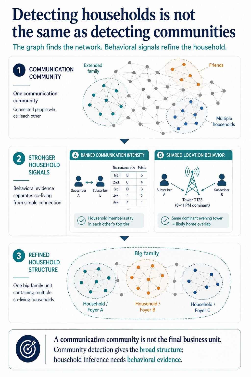
Detecting households is not the same as detecting communities. This project started from precomputed telecom communication communities and refined them into two nested levels of social structure: Big Family (extended social unit) and Foyer / Household (likely co-living unit). A tie had to satisfy both communication closeness and persistent shared cell-tower usage to qualify as a household candidate.
Architecture
The Problem
The project started from precomputed communication communities derived from call graph analysis. Those communities identified groups of subscribers who call each other frequently — but for CVM purposes, that output was too coarse. A communication community can mix extended family, multiple households, close friends, and work relationships all in one cluster.
The real goal was to identify likely household-level ties inside those broader communities — the smaller co-living unit that drives actual shared purchasing decisions and family offer targeting. The project refined the graph output into two nested social structures:
- Big Family: the broader connected social unit (extended family)
- Foyer / Household: the smaller likely co-living unit inside it
Key insight: The first graph segmentation is often not the final business unit. Detecting households requires a second refinement layer on top of community detection.
Behavioral Signal Design
To qualify as a household-level tie, two conditions had to be satisfied simultaneously. Neither alone was sufficient.
Signal 1: Ranked Communication Intensity
Build top-5 incoming and outgoing contact lists for each subscriber, preserving ordinal importance. A household tie is more likely if the other person appears in the top contacts — not just if they have any calls together. Ranked lists filter out occasional contacts and focus on persistent, close relationships.
Signal 2: Shared Cell-Tower Usage
Dominant cell-tower usage is a behavioral proxy for recurring location overlap. Instead of asking where people declared they lived, the pipeline inferred shared daily-life proximity from repeated infrastructure traces — the top 5 most-used towers per subscriber. A household tie requires shared dominant towers, not just shared calls.
Signal Intersection: Both Must Hold
A tie is classified as a household candidate only if the related subscriber appears in both the top contact list AND shares dominant cell-tower locations. Communication closeness without shared location could be a work relationship. Shared location without communication closeness could be neighbors. Only the intersection reliably points to a household structure.
Pipeline: Key SQL Steps
Filter to communities with enough telecom subscribers
select community_candidates.*,
       community_sizes.telecom_member_count
from community_candidates
left join (
    select community_id,
           count(subscriber_id) as telecom_member_count
    from community_candidates
    group by community_id
) community_sizes on community_candidates.community_id
                   = community_sizes.community_id
where community_sizes.telecom_member_count >= 2;
Aggregate direct subscriber-to-subscriber communication
select caller_subscriber_id   as source_subscriber_id,
       callee_subscriber_id   as target_subscriber_id,
       sum(call_count)        as total_calls,
       sum(call_duration) / 60 as total_duration_minutes,
       sum(active_days)       as total_active_days
from subscriber_traffic
where source_is_telecom_customer = 1
  and target_is_telecom_customer = 1
group by caller_subscriber_id, callee_subscriber_id;
Keep top-used cell towers per subscriber (proxy for home location)
select * from (
    select subscriber_cells.*,
           row_number() over (
               partition by community_id, subscriber_id
               order by tower_usage_count desc
           ) as tower_rank
    from subscriber_cells
)
where tower_rank <= 5;
Keep ties that are both close contacts AND share dominant location
case
  when related_subscriber_id in (
       top_outgoing_contact_1,
       top_outgoing_contact_2,
       top_incoming_contact_1,
       top_incoming_contact_2
  )
  then related_subscriber_id
end as close_contact_subscriber_id
Graph partitioning in R (igraph) to produce Foyer groups
select distinct
       subscriber_id             as source_subscriber_id,
       substr(household_id, 1, 8) as target_subscriber_id,
       big_family_id              as family_group_id
from household_graph_edges
where household_id is not null
order by big_family_id;
Key Takeaway
Cell-tower dominance as a behavioral proxy for home-location overlap is one of the most useful patterns in applied telecom analytics. Instead of asking where people declared they live, the pipeline infers shared daily-life proximity from repeated infrastructure traces. The strongest features are not always direct measurements — sometimes they are operational traces that behave like reliable proxies for the concept you care about.
Design insight: The first clustering step is often only the beginning. In graph analytics, the real work starts when you refine a connected community into the smaller behavioral unit the business actually needs — and that requires a second signal layer beyond call frequency alone.